Sonja Spitzer & Claudia Reiter

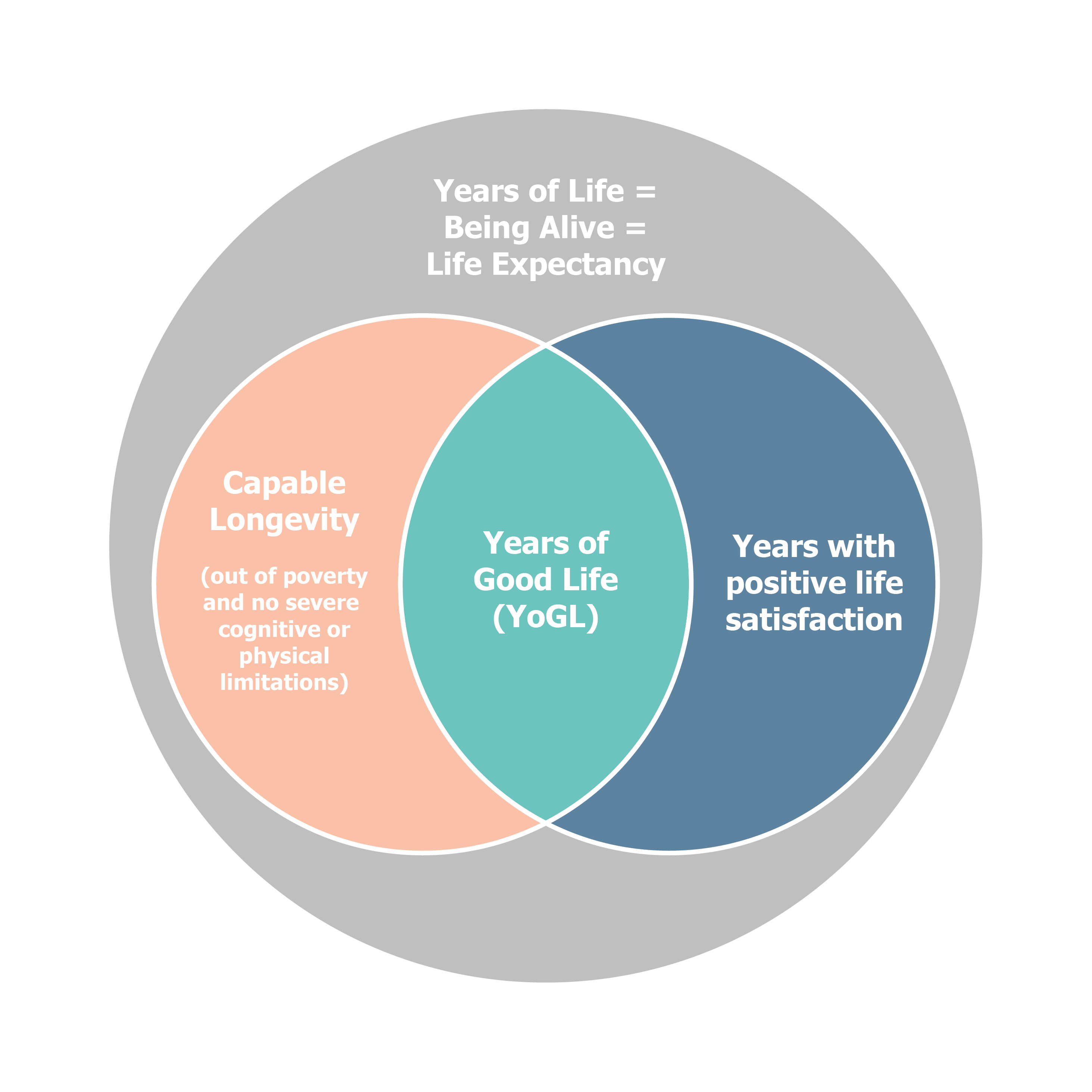
Years of Good Life (YoGL) is a newly developed indicator that takes a demographic approach to directly measure multi-dimensional human well-being and its change over time. Its trend over time for any sub-population can also be used as criterion to assess whether development is sustainable once feed-backs from environmental changes are factored in. In order to enjoy any quality of life, one has to be alive; but since mere survival does not capture well-being, ‘years of good life’ are made conditional on meeting minimum standards as depicted in the circular chart. Years of life are counted as ‘good’ if they are spent above a threshold with respect to objectively observable conditions (being out of poverty, being without cognitive limitations, and having no serious physical disabilities), as well as subjective life satisfaction.

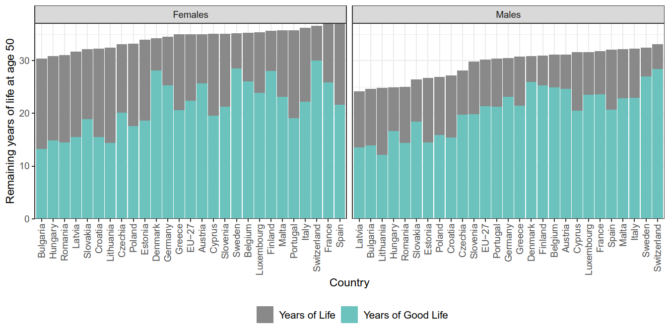
In Europe, YoGL varies considerably between countries – particularly for older age groups. In 2017, Swiss men aged 50 could expect to live another 33.1 years, of which 28.5 are considered ‘good’ years (86%). By contrast, Lithuanian men of the same age could only expect to live another 24.8 years, of which only 12.1 years are considered ‘good’ years (49%). Generally, Southern and Western European countries such as Spain, Italy, France, and Switzerland have exceptionally high life expectancy at age 50. However, it is mostly Northern European countries, but also Switzerland and Belgium, whose populations are expected to spend their remaining life years to a great extent in good years. Central and Eastern European countries have both low life expectancy and low YoGLs. While male life expectancy is consistently lower than female life expectancy, gender differences in YoGL are less pronounced: YoGL at age 50 for the EU-27 in 2017 was 22.4 for females (life expectancy of 35 years) and 21.4 for males (life expectancy of 30.2 years).

References:
Lutz, W., Lijadi, A., Strießnig, E., Dimitrova, A., and Caldeira Brant de Souza Lima, M. (2018). Years of Good Life (YoGL): A new indicator for assessing sustainable progress. IIASA Working Paper, WP-18-007.

Reiter, C., and Lutz, W. (2020). Survival and Years of Good Life in Finland in the very long run. Finnish Yearbook of Population Research, 54, 1–27. https://doi.org/10.23979/fypr.87148

Tomáš Sobotka and Kryštof Zeman

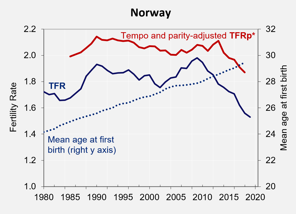
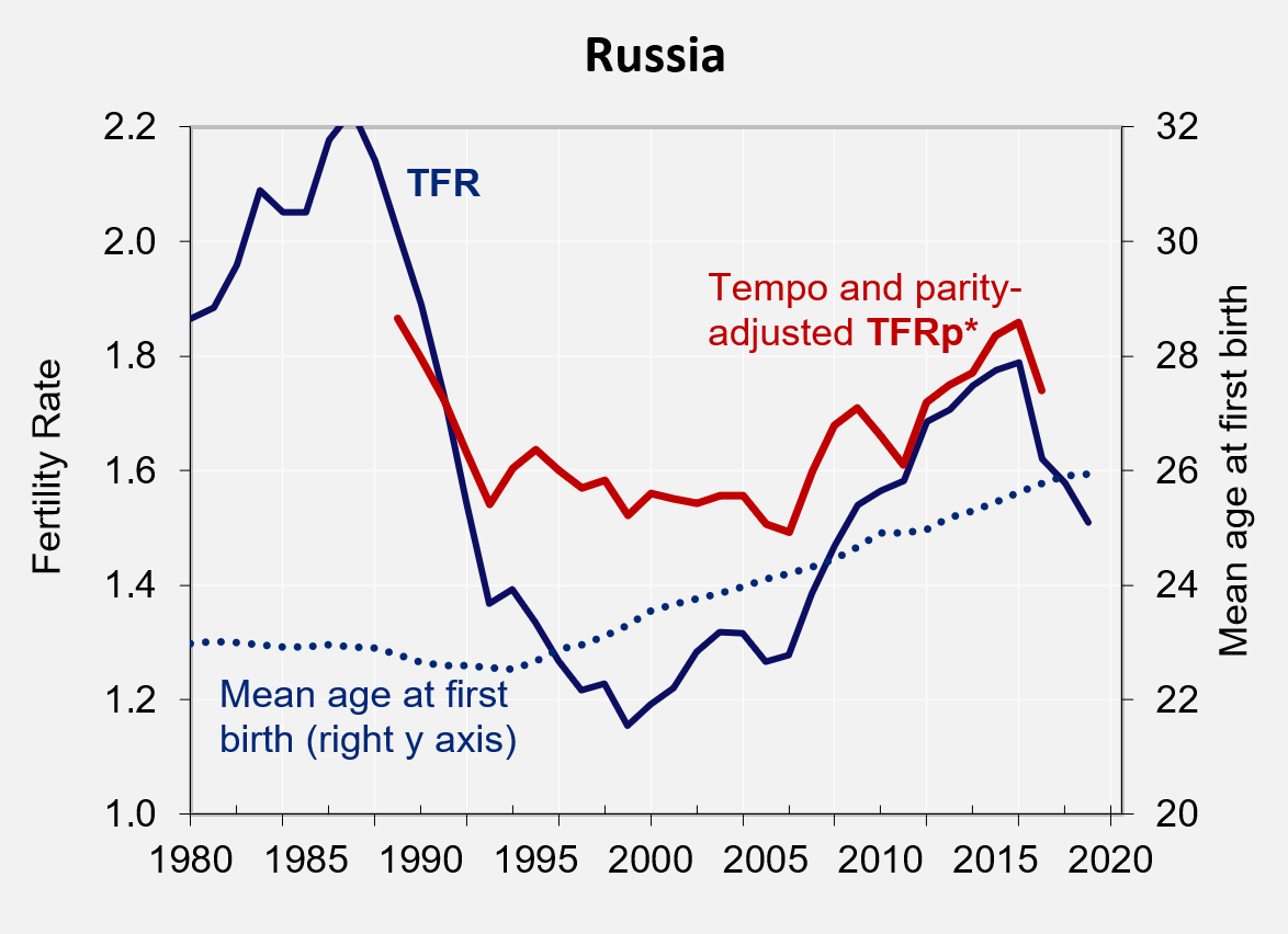
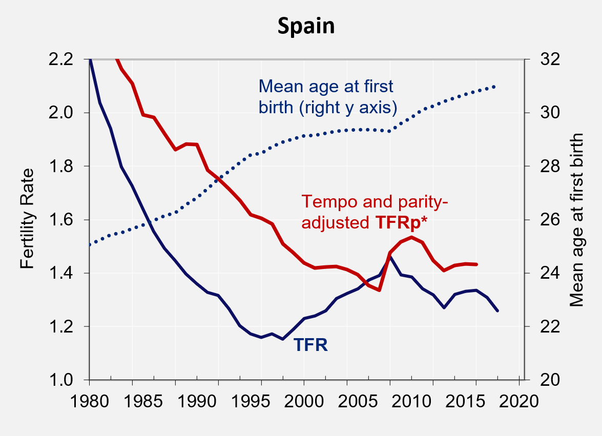
Fertility over a given time is commonly measured by the Total Fertility Rate (TFR). However, TFR is sensitive to changes in the average age of childbearing, which has been rising in Europe for several decades. As births shift to later ages, they are both postponed into the future and spread over a longer period of time. This ‘stretching’ of reproduction results in a depressed period TFR, even if the number of children that women have over their lifetimes does not change.

Alternative indicators to TFR have been developed to provide a more accurate measure of the mean number of children per woman in a calendar year. Here we use Tempo- and Parity-adjusted Total Fertility (TFRp*; Bongaarts and Sobotka 2012), which is based on age- and parity-specific fertility rates, as well as changes in mean ages at birth. When available, this data sheet displays the TFRp* of 2016. For countries lacking the required data, we use Tempo-adjusted TFR (TFR-BF) proposed by Bongaarts and Feeney (1998), averaged over the 3-year period of 2015–2017.

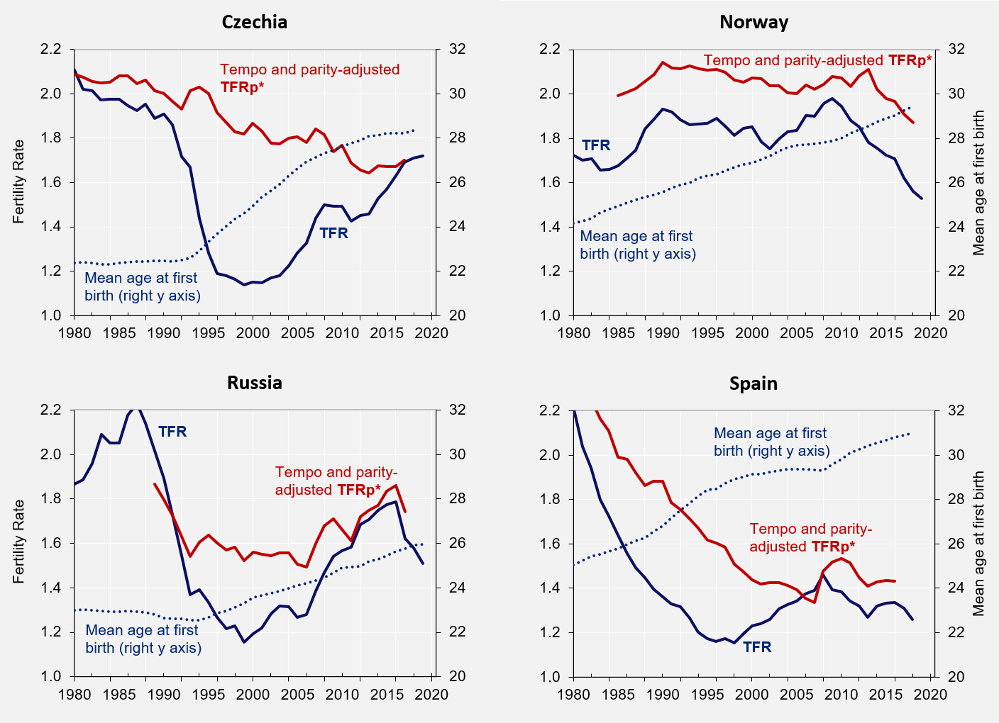
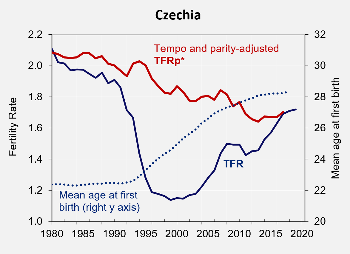
The graphs compare conventional TFR and TFRp* from 1980–2019 in four countries with different fertility patterns: Czechia, Norway, Russia and Spain. They also show the rise in the mean age at first birth. In some cases fertility postponement has resulted in unstable (‘roller-coaster’) TFR trends and a huge gap between conventional and tempo-adjusted fertility, especially in Czechia in the late 1990s when the TFR fell below 1.2, while the TFRp* stayed above 1.8. This decrease in TFR was followed by a robust recovery in the last two decades, when it converged with the TFRp* at 1.7 in 2017. For Russia, data suggest that pro-natalist policies introduced in 2006 had a strong effect, although more on conventional TFR (and thus also on the timing of births) than on the tempo- and parity-adjusted TFRp*. The fertility boost given by pro-natalist policies has recently lost its steam, with the TFR and TFRp* plummeting after 2015.

By contrast, the TFR in Spain and Norway started falling earlier, soon after the start of the Great Recession in 2008. In Spain, this slide was briefly interrupted around 2013–2015, but in Norway it continued until 2019, resulting in a lowest-TFR on record. The TFRp* also followed a downward trend, albeit milder than the conventional TFR. This suggests that the TFR declines have reflected a renewed postponement of fertility (especially of first births), as well as a fall in family size. A similar trend has taken place in many other countries across Europe, especially in Southern Europe, Nordic countries, and parts of Western Europe.

Figure Notes:
Figure 1: Fertility trends in Czechia, 1980–2019
Figure 2: Fertility trends in Norway, 1980–2019
Figure 3: Fertility trends in Russia, 1980–2019
Figure 4: Fertility trends in Spain, 1980–2018

References:
Bongaarts, J. and G. Feeney 1998. On the quantum and tempo of fertility. Population and Development Review 24(2): 271–291.

Bongaarts, J. and T. Sobotka 2012. A demographic explanation for the recent rise in European fertility. Population and Development Review 38(1): 83–120.

Tomáš Sobotka and Kryštof Zeman

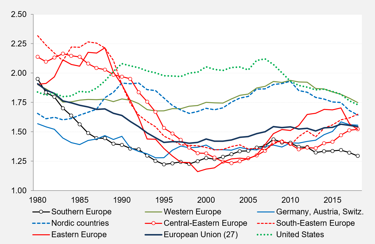
Following turbulent changes in period fertility in the 1980s and 1990s, when fertility declined in many regions, a North-West vs. South-East divide emerged. Northern and Western Europe (aside from the German-speaking countries) had moderately low fertility rates, with the period Total Fertility Rate (TFR) at 1.7–2.0. All other regions in Europe had low or very low TFR, typically reaching between 1.2 and 1.4. This regional differentiation was retained during the period of gradual recovery in fertility during the 2000s.

However, this fertility divide began to unravel during the Great Recession in 2008-13, as different regions took contrasting fertility paths that often continued after the recession had ended.

Period TFR increased vigorously in Eastern Europe, supported by pronatalist policies in Russia, Belarus and Ukraine before taking a dip in 2017–2019. Fertility also recovered in Central-Eastern Europe, South-Eastern Europe as well as in Austria, Switzerland and Germany, where it stays close to the highest levels since the 1970s. By contrast, the TFR declined over the last decade in Western Europe and in the Nordic countries, bringing their fertility well below the peaks reached around 2008–2010. Several countries including Ireland, Finland and Norway reached their lowest TFRs on record in 2018, in part due to a renewed postponement of first births to later ages (see Box on tempo effect and adjusted fertility). Outside Europe, a similar downturn in fertility to a record-low level has taken place in the United States. After a brief stabilization, fertility also declined further in Southern Europe: with an average TFR just below 1.3, Southern Europe has emerged as the lowest-fertility region in Europe.

These contrasting regional trends in recent years have led to the narrowing of regional and cross-country fertility differences across the continent. The TFR in most parts of Europe now occupies the previously “empty” middle position, around 1.4–1.7.

Figure Notes:
Figure: Total Fertility Rate (TFR) in European regions and the United States, 1980–2018

Vanessa di Lego

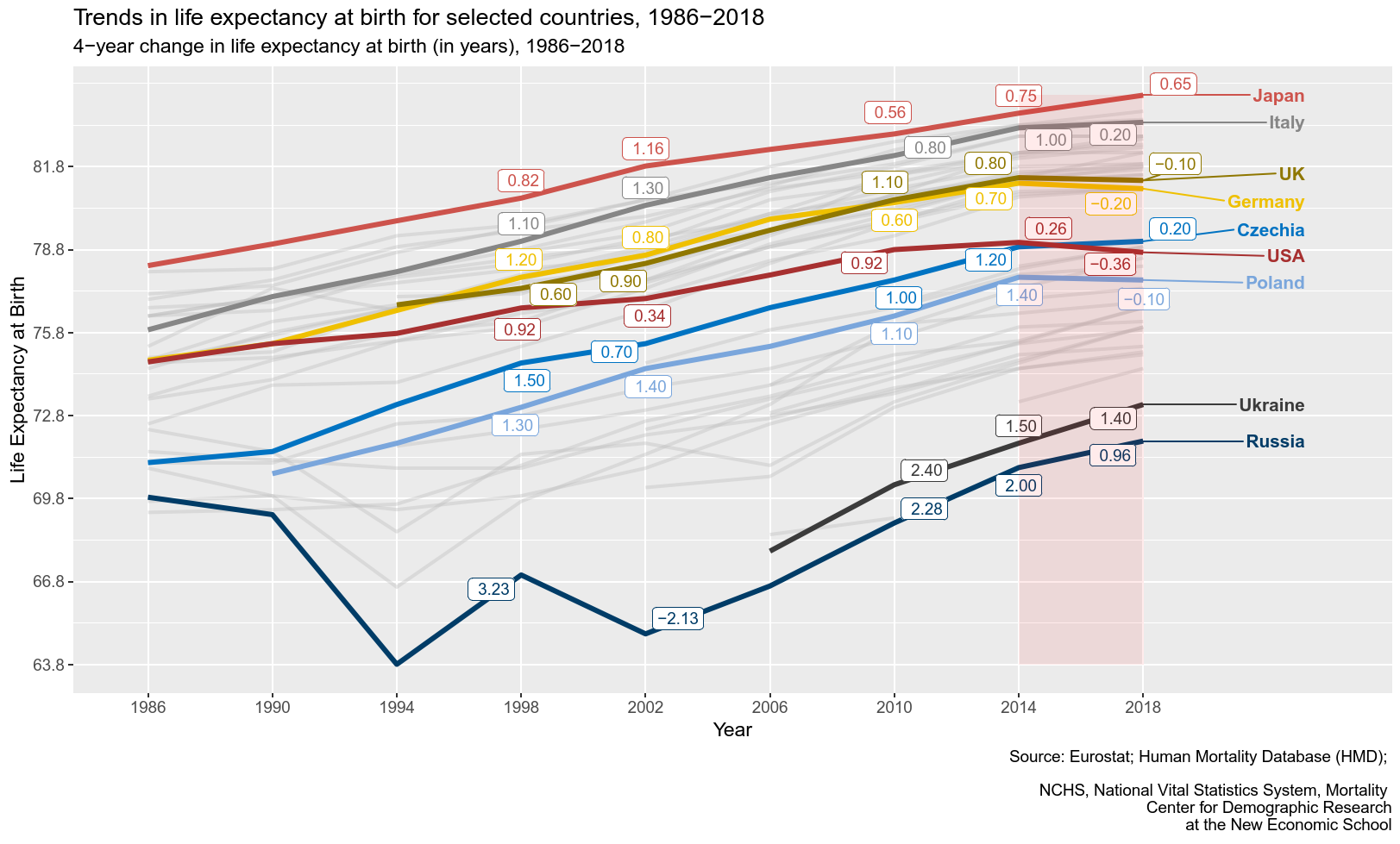
Many highly developed countries have experienced decelerating improvements or even slight declines in life expectancy. How did this trend evolve over time and between countries? The figure shows the trends in Total Period Life Expectancy at birth (hereby called TPLE) for selected European countries, together with Japan and the United States from 1986 until 2018, with the labels highlighting a 4-year interval of absolute change in TPLE. The overall trajectory since 1986 is one of consistent increase in TPLE, with the exception of countries - like Russia - that experienced profound discontinuities in their gains after the fall of the Berlin Wall, consistently improving their TPLE only after 2002. Breaking from the general trend, the pace of increase in Japan and Italy started to slow down in the 2000s. More recently, in 2014-2018, most countries recorded a dramatic deceleration in their gains, with Germany, United Kingdom, United States, and Poland even reporting declines in TPLE. This trend has brought attention to the causes of TPLE stagnation, commonly interpreted as an indication of failing to improve mortality rates. However, the evidence does not allow such a straightforward interpretation.

First, patterns in age- and cause-of-death that bring stagnation in TPLE vary between countries. While in Japan, Italy, UK and Germany, the primary driver is mortality at older ages (65+), in the United States it is mortality of people below age 65. Deaths related to respiratory, cardiovascular, Alzheimer’s and other nervous system diseases explain most of these trends for European countries, whereas external causes and opioid drug overdose had the largest impact in the United States (Ho and Hendi 2018). In addition, seasonal fluctuations in flu waves affect TPLE trends, with below-average mortality in 2014 and the excess mortality in 2015 impacting the trend in the last decade. Lastly, the TPLE is a period measure of the average number of years that a hypothetical cohort of newborns is expected to live, should current age-specific death rates remain constant. However, current age-specific death rates do not necessarily capture pure period events and are sensitive to cohort, heterogeneity, and tempo effects, possibly leading to temporary inflation or deflation of TPLE (Luy et al. 2019; Peters, Nusselder, and Mackenbach 2014; Vaupel 2008). Hence, further research is needed to determine the extent to which diminished gains in the TPLE are the result of worsening health conditions, past progress in survival, or a shifting of deaths.

References:
Ho, Jessica Y, and Arun S Hendi. 2018. 'Recent Trends in Life Expectancy across High Income Countries: Retrospective Observational Study.' BMJ, August, k2562. https://doi.org/10.1136/bmj.k2562.

Luy, M, P Di Giulio, V Di Lego, P Lazarevič, and M Sauerberg. 2019. “Life Expectancy: Frequently Used, but Hardly Understood.” Gerontology. https://doi.org/10.1159/000500955.

Murphy, M., M. Luy, and O. Torrisi. 2019. 'Mortality Change in the United Kingdom and Europe.' Social Policy Working Paper 11-19. London.

Peters, Frederik, Wilma J. Nusselder, and Johan P. Mackenbach. 2014. 'Tempo Effects May Distort the Interpretation of Trends in Life Expectancy.' Journal of Clinical Epidemiology 67 (5): 596–600. https://doi.org/10.1016/j.jclinepi.2013.07.020.

Vaupel, James W. 2008. 'Turbulence in Lifetables: Demonstration by Four Simple Examples.' In How Long Do We Live?, 271–79.

Claudia Reiter, Dilek Yildiz, Caner Özdemir & Anne Goujon

Attending school does not necessarily equate to learning. However, efforts to merge qualitative and quantitative measures of human capital are so far rare and have only covered a limited number of countries or focused solely on skills measured with school tests. To remedy that, the Wittgenstein Centre for Demography and Global Human Capital has started a new initiative to provide a global historical database for Skills-Adjusted Mean Years of Schooling (SAMYS) of adults.

Quantitative data on years of schooling are merged with qualitative adult skills assessments, such as the OECD’s PIAAC or the World Bank’s STEP Skills Measurement Program, to obtain a measure of human capital that considers both access to and outcomes of education. To make SAMYS comparable across countries and over time, the 2015 population-weighted OECD average PIAAC literacy score is used as the standard of comparison. Accordingly, a skills adjustment larger than 1 means the respective country doing better than the OECD average. If the skills adjustment is below 1, the opposite is true: the skills of people correspond, on average, to fewer years of schooling than they actually went through when compared with OECD average.

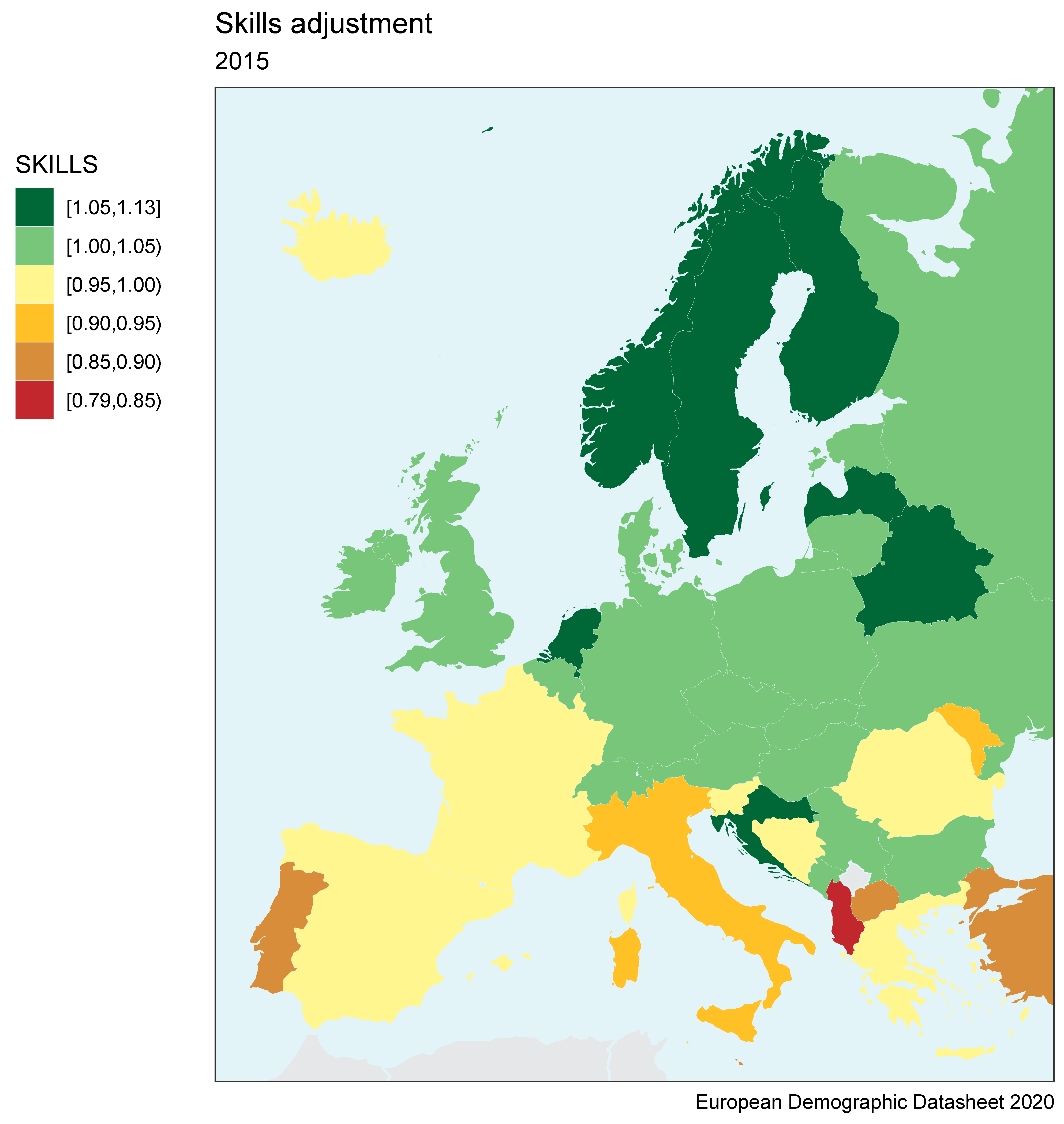
The map below depicts the estimated skills adjustment for the population aged 20-64 in Europe in 2015 – without considering the mean years of schooling for each country. The composite indicator, SAMYS, is included in the data table on the front side.

Results reveal a considerable North - South divide in Europe. Nordic countries and some Post-Soviet countries (notably Latvia, Belarus, Estonia, and Russia) perform comparably well in large-scale literacy assessments. By contrast, human capital is lagging behind in terms of skills formation in the countries in South-Eastern Europe and in the Caucasus region, but also in Portugal, Italy, and Spain. Particularly low values were estimated for Albania, Malta, and Turkey – in all three countries the average skills level, adjusted for the years of schooling received, constitutes only 80-85% of the OECD average.

Figure Notes:
For those countries, where no empirical adult assessment data exist, our estimates are based on a regression model taking into account educational attainment, adult illiteracy rates, old-age dependency ratios, and years (time).

References:
Reiter, C., Özdemir, C., Yildiz, D., Goujon, A., Guimaraes, R., and Lutz, W. (2020). The Demography of Skills-Adjusted Human Capital. IIASA Working Paper WP-20-006. Laxenburg, Austria. Available at: http://pure.iiasa.ac.at/id/eprint/16477/

Francisco Rowe, Martin Bell, Aude Bernard, Elin Charles-Edwards

With the decline of spatial variations in fertility and mortality rates, internal migration has now become the primary demographic process shaping the distribution of populations within countries. Globally, internal migration outnumbers international migration by a factor of 4 to 1 (Bell et al 2015). While growing attention has been dedicated to international migration, migration between regions within countries remains less well understood. The general dearth of internal migration studies, data, and indicators can be traced to the complexities of human mobility and the absence of internationally agreed standards for the collection and measurement of internal migration data. Thus, while comparative indicators of fertility and mortality are routinely reported, statistical indicators of internal migration are conspicuous by their absence.

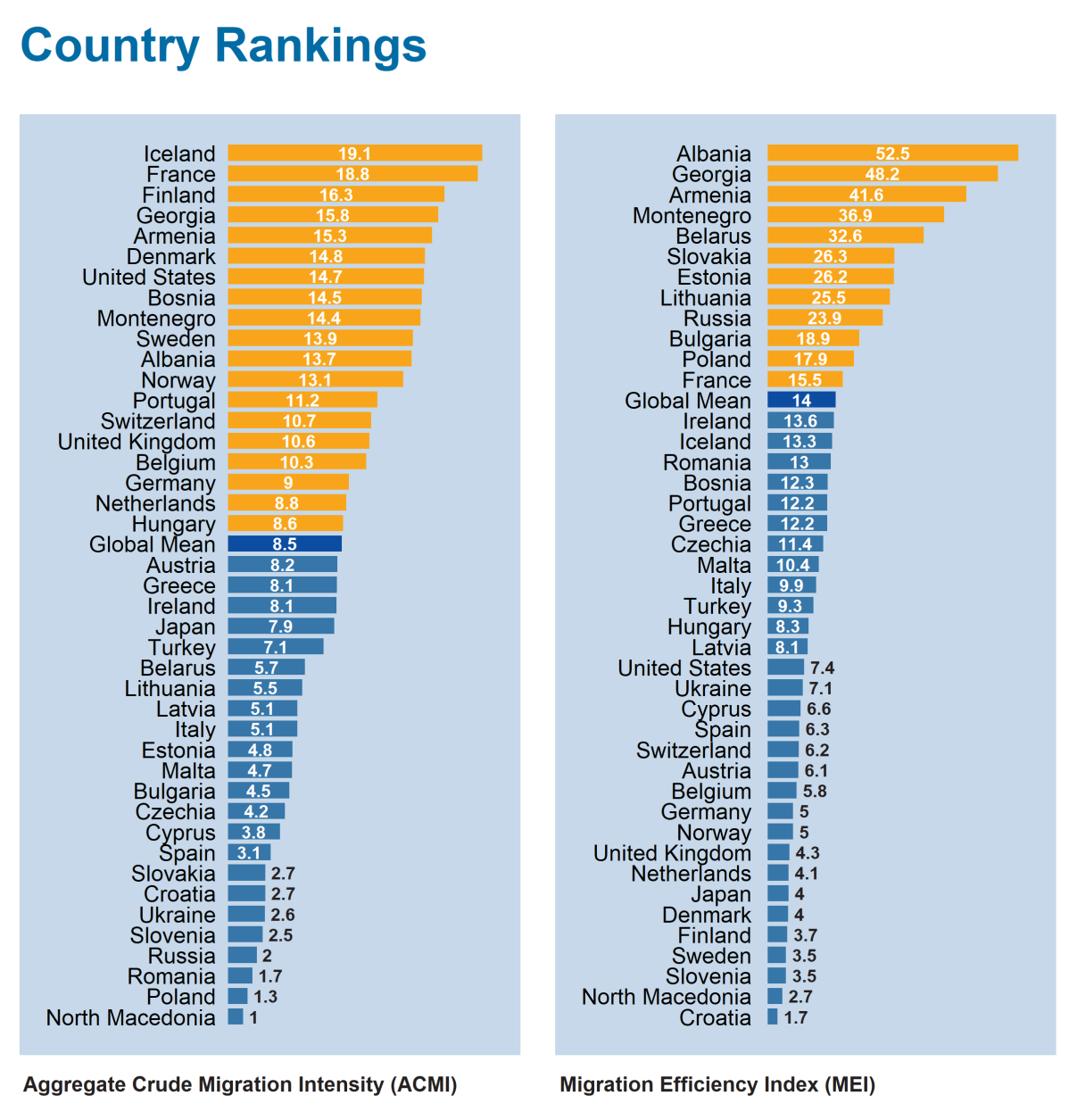
In recent years, significant progress has been made in developing a rigorous framework for cross-national comparisons of internal migration, particularly through the IMAGE project (Internal Migration Around the GlobE), which (1) proposed a suite of statistical indicators, (2) developed methods to generate estimates where these metrics are not collected directly, and (3) made cross-national comparisons using a global repository of data. The Aggregate Crude Migration Intensity (ACMI) and the Migration Effectiveness Index (MEI) are two of these indicators.

The ACMI captures the intensity of internal migration, measuring all changes of residential address in a given interval. Few countries collect this information directly, but the IMAGE project generated robust estimates by measuring migration rates at multiple random geographical scales using the method proposed by Courgeau et al (2012). The MEI, which ranges from 0 to 100, quantifies the balance between regional flows and counterflows, with low values indicating largely reciprocal exchanges between regions, and high values suggesting strongly directional flows. Measured at multiple geographical scales, MEI values are remarkably stable with scale when computed for 20 regions or more (Rees et al 2017). Together, intensity and effectiveness drive the redistributive impact of internal migration on national populations.

The ACMI varies widely across Europe. It ranges from just over 1% per annum in Macedonia to over 18% in France and Iceland, with levels close to the global mean in Hungary and Austria. A clear geographical pattern underpins these variations, ranging from high intensities in Nordic and Western European countries, including the United Kingdom, to low intensities in Southern and Eastern Europe, including Spain, Italy, and former members of the Soviet Union. Internal migration can be shaped by interaction with international migration by intensifying mobility to getaway cities, which may account for the higher than expected levels of internal migration in Georgia, Armenia, Albania, Bosnia-Herzegovina, and Montenegro.

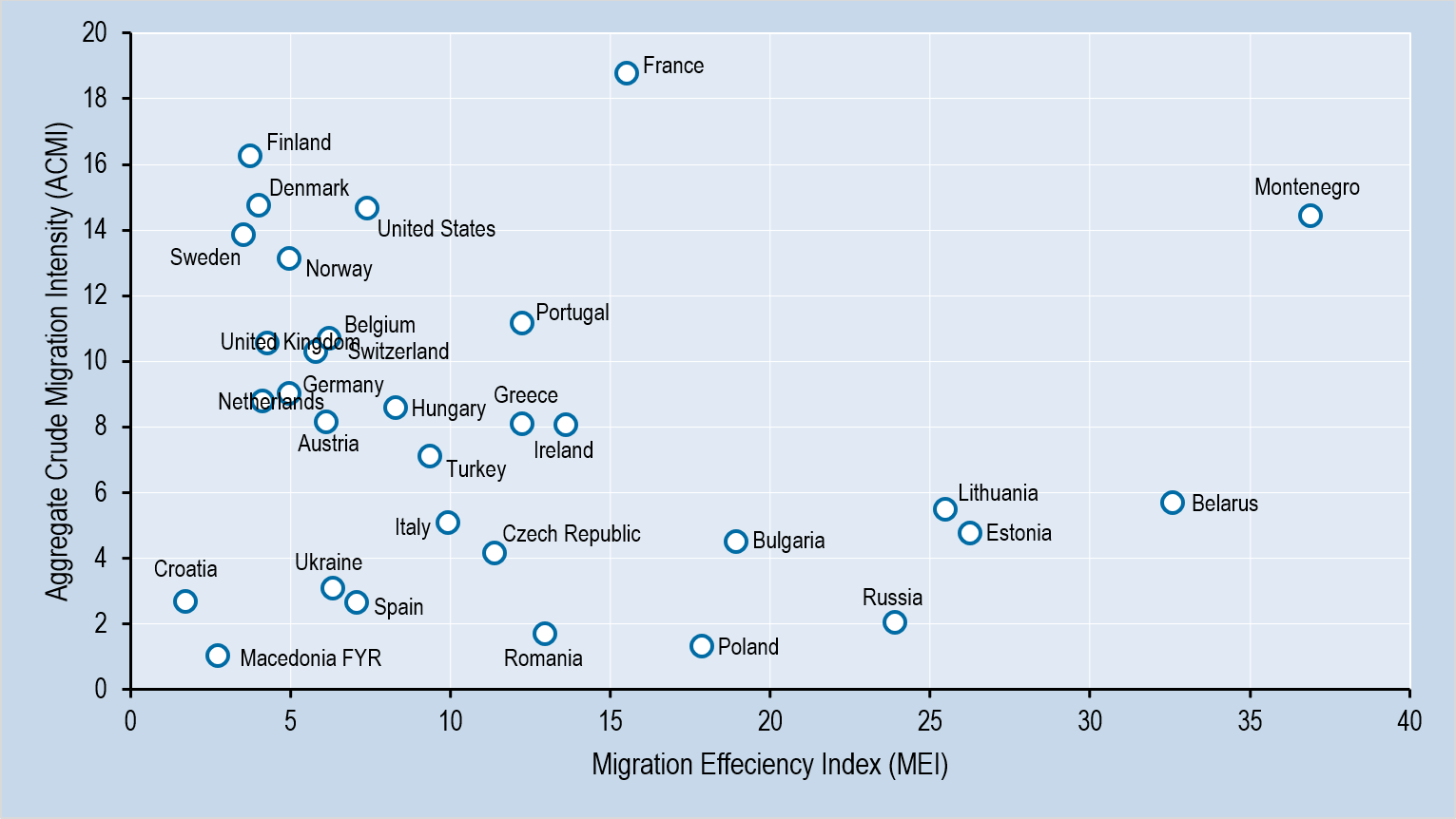
Ranking countries by their MEI values reveals a moderate inverse relationship with the ACMI (Pearson r=-0.41) when outliers are removed (France and Montenegro). In countries where migration intensities are high, inter-regional flows tend to be closely balanced, whereas many of those with low migration intensities are undergoing higher levels of redistribution. At a global scale accumulating evidence suggests these patterns are driven by complex links with economic development, external migration, and a range of social and demographic variables.

In Northern and Western Europe, the redistributive impact of high internal migration intensity is moderated by low levels of migration effectiveness (closely balanced flows) (Rowe et al., 2019). By contrast, migration in the South and East tends to be highly asymmetrical, but its impact on population redistribution is offset by low migration intensity. Deviating from this general pattern are marked exceptions, for example, France and Montenegro, where the ACMI and MEI are both high.

Figure Notes:
Figure 1: Measure of the Intensity and Impact of Internal Migration. ACMI measures all changes of residential addresses over a one-year interval. MEI measures the degree of balance between internal migration flows and counter flows. MEI is reported for countries with data for 20 regions or more.
Figure 2: The Relationship between the Intensity and Effectiveness of Internal Migration. Only countries with data for 20 regions or more are reported.

References:
Bell, M., Charles-Edwards, E., Ueffing, P., Stillwell, J., Kupiszewski, M. and Kupiszewska, D. (2015) Internal migration and development: comparing migration intensities around the world. Population and Development Review, 41(1), pp.33-58. https://doi.org/10.1111/j.1728-4457.2015.00025.x

Courgeau, D., Salut M., and Bell, M. (2012) Estimating changes of residence for cross-national comparison. Population 67(4), pp.631-651.

Rees, P., Bell, M., Kupiszewski, M., Kupiszewska, D., Ueffing, P., Bernard, A., Charles-Edwards, E. and Stillwell, J. (2017) The impact of internal migration on population redistribution: An international comparison. Population, Space and Place, 23(6), p.e2036. https://doi.org/10.1002/psp.2036

Rowe, F., Bell, M., Bernard, A., Charles-Edwards, E. and Ueffing, P. (2019) Impact of Internal Migration on Population Redistribution in Europe: Urbanisation, Counterurbanisation or Spatial Equilibrium? Comparative Population Studies, 44, pp.201-233. https://doi.org/10.12765/CPoS-2019-18en

Bernhard Binder-Hammer

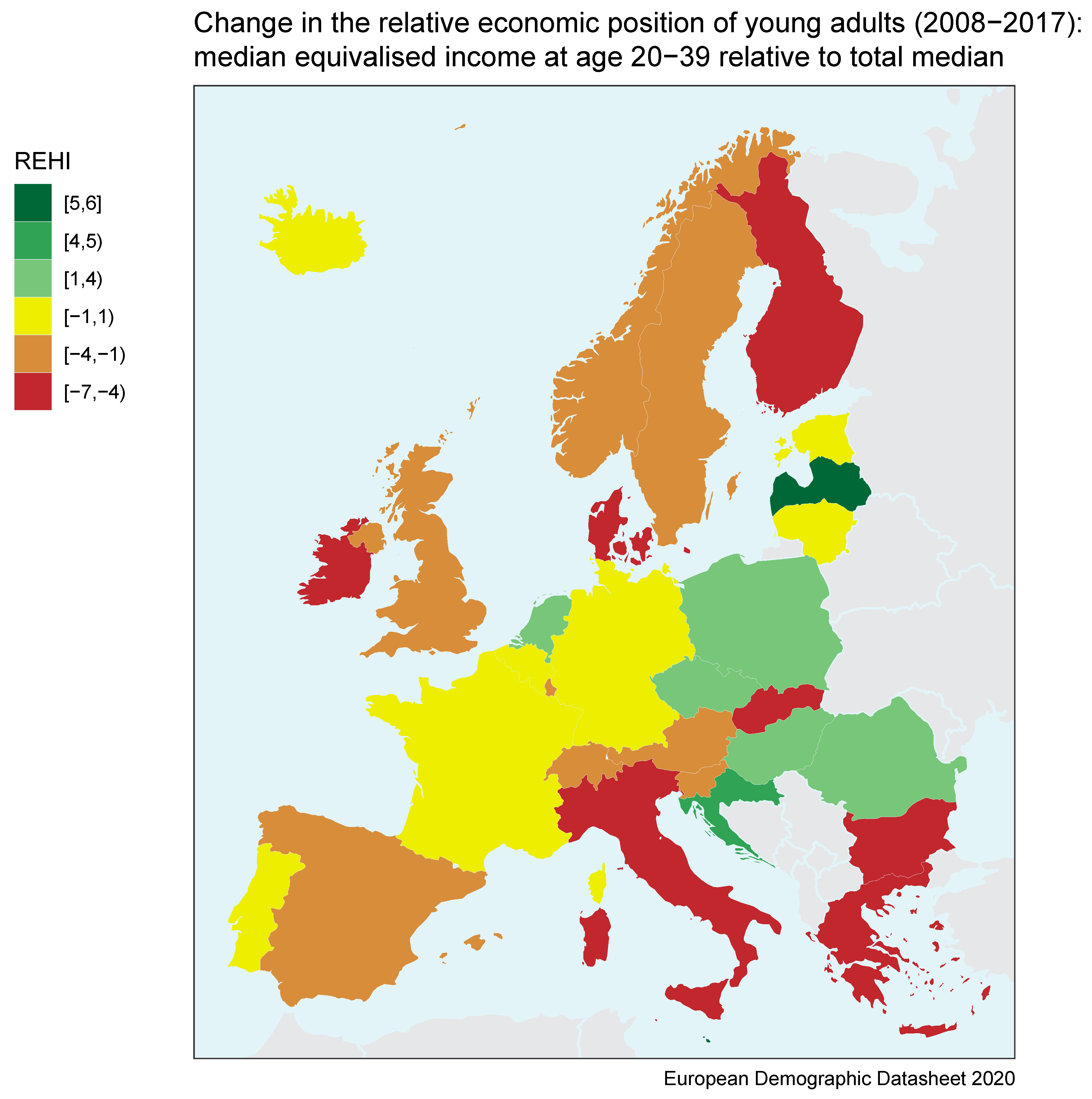
The 2008 financial crisis hit the income of younger generations much harder than the income of older persons. A deteriorating economic situation for young persons has many undesired consequences, such as a further reduction of fertility and an increase in poverty of young family households. Therefore, monitoring economic well-being from a generational perspective is indispensable for a meaningful evaluation of social protection systems.

Equivalised Household Income (EHI) is frequently used for the evaluation of economic well-being. EHI measures the income of households relative to the number of effective consumers, accounting for economies of scale in consumption and lower consumption of children compared to adults. The first adult household member is counted as a full effective consumer, further adult members represent 0.7 effective consumers, and children below the age of 14 are counted as 0.3 effective consumers. A huge advantage of EHI is accessibility due to its collection in EU-SILC for 32 European countries. One disadvantage of EHI is that it assumes equal sharing of income among household members. Therefore, EHI disregards the differences in income changes between adult generations who live in the same household.

The change in age-specific real EHI between 2008 and 2017 is an indicator of how the financial crisis and the sovereign debt crisis impacted the economic well-being of different age groups. Based on this indicator, economic well-being among younger people aged 20-39 fell in every third country (in 10 out of 31) between 2008 and 2017. Young adults in Greece experienced the strongest fall in real EHI at 40%. Note that EHI is measured in Euros. For countries that are not members of the euro zone the changes in EHI also reflect changes in the exchange rate of the local currency against Euro (which explains the high increase in Switzerland).

The economic crises and developments during the period 2008-2017 resulted in a reallocation of income from young to old in most countries. Declines in the relative economic position of young people are illustrated by the map of change in EHI at ages 20-39 relative to the median of the total adult population. The relative EHI of young people declined in 23 countries, including all countries in Western, Southern and Northern Europe, except the Netherlands. This decline was most pronounced in Italy, Greece, Bulgaria, Ireland, Denmark and Slovakia, where median EHI at ages 20-39 dropped by more than 4% compared to the total median.

Figure Notes:
Figure 1: Changes in the relative economic position of young adults (2008-2017): median equivalised income at age 20-39 relative to total median

David E. Bloom, Victoria Y. Fan, Vadim Kufenko, Osondu Ogbuoji, Klaus Prettner, Gavin Yamey

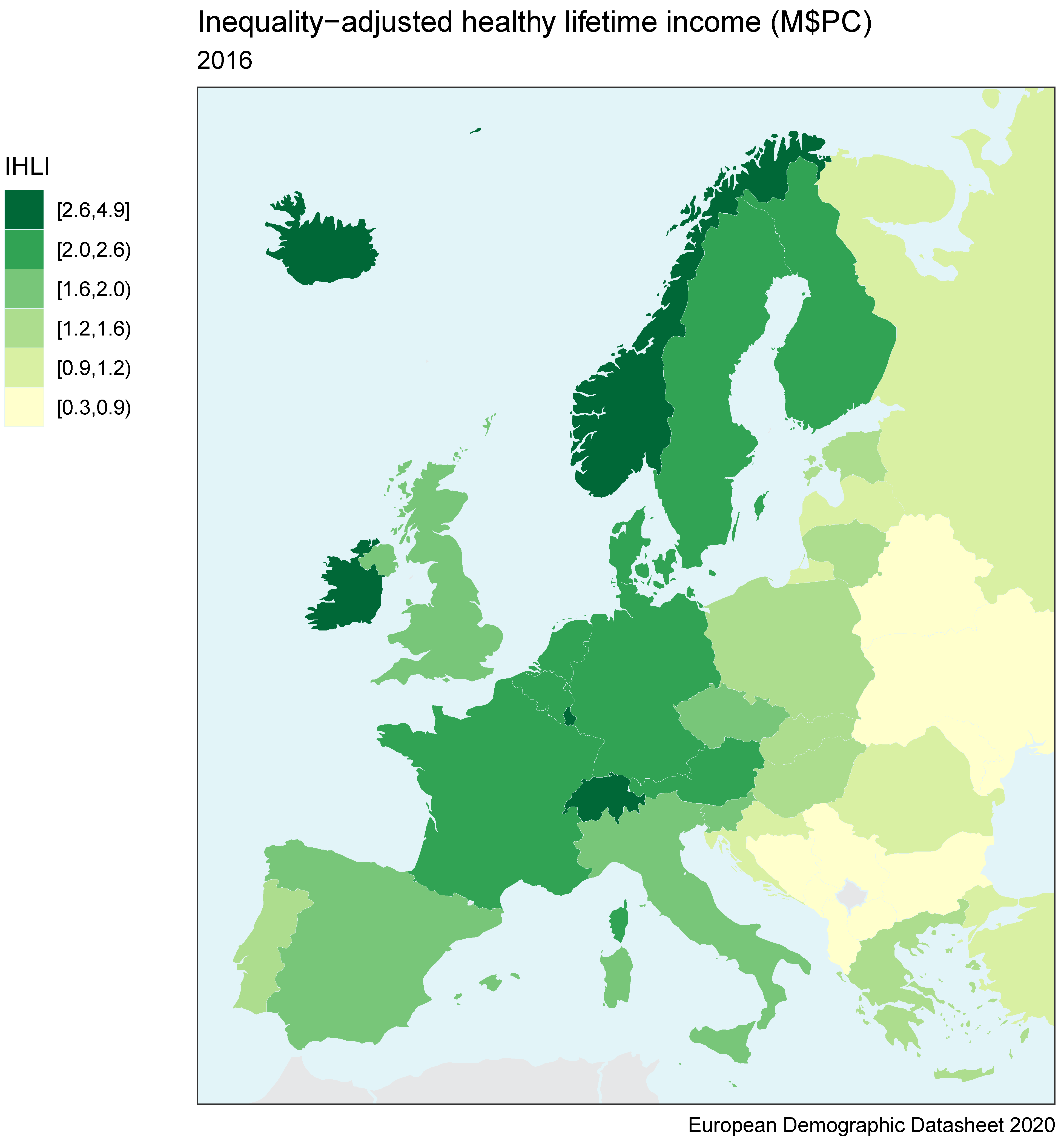
Per capita GDP is of limited use as a welfare measure because – among other shortcomings – it disregards the benefits of living long and healthy lives and it does not adjust for inequality (Sen, 1976; Fitoussi et al., 2009; Fan et al., 2018). In Bloom et al. (2020), we propose inequality-adjusted healthy lifetime income (IHLI) as a remedy for these two issues. IHLI consists of three components: i) GDP per capita adjusted for purchasing power (pppGDPpc) to capture material well-being, ii) healthy life expectancy at birth (HALE) to capture the benefits of living long and healthy lives (and thereby some of the effects of environmental quality), and iii) an inverse measure of the Gini coefficient (1 − Gini) to take inequality into account. Our indicator is defined in a straightforward manner as:

IHLI_i = pppGDPpc_i × HALE_i × (1 - Gini_i)

This formulation implies the straightforward interpretation of IHLI_i being the income that a newborn in country i can expect to earn over the years in which she is in good health, for the given economic and health conditions in country i, and adjusted for the level of inequality. Note that the unitary weights of the different components in this formulation follow mathematically from the interpretation of the indicator and the units of measurement of the subcomponents.

IHLI has the following advantages over other alternatives to per capita GDP, such as the Human Development Index (HDI):

IHLI has an immediately interpretable economic value,
The weighting of its components follows mathematically from the interpretation of the indicator and the units in which the subcomponents are measured,
IHLI does not depend on aggregating different sub-indicators that are based on incompatible units of measurement,
IHLI is not restricted to a value between zero and one and is thus not bounded from above,
IHLI is parsimonious in terms of computation and data input requirements,
IHLI can readily be obtained for many different countries.

We compute the indicator for the countries in the European Demographic Datasheet using the following sources: Solt (2019) for the Gini index of disposable incomes, World Bank (2019) for pppGDPpc, and World Health Organization (2019) for HALE. The results are displayed in Figure 1.

References
Bloom D.E., Fan V.Y, Kufenko, V., Ogbuoji O., Prettner K., and Yamey G. (2020). Going beyond GDP with a parsimonious indicator: Inequality-Adjusted Healthy Lifetime Income. Hohenheim Discussion Papers in Business, Economics and Social Sciences, WP 01-2020, Stuttgart, Germany. Available at: https://ideas.repec.org/p/zbw/hohdps/012020.html

Fan V.Y., Bloom D.E., Ogbuoji O., Prettner K., and Yamey G. (2018). Valuing health as development: going beyond gross domestic product, The BMJ, 363: k4371.
Fitoussi J.P., Sen A., and Stiglitz J. (2009). Report by the commission on the measurement of economic performance and social progress. The Commission on the Measurement of Economic Performance and Social Progress. Paris, France.

Sen (1976). Real National Income. The Review of Economic Studies, 43(1): 19–39.

Solt F. (2019). Measuring income inequality across countries and over time: the standardized world income inequality database. SWIID Version 8.2, November 2019. Available at https://fsolt.org/swiid/ [Accessed on January 20, 2020].

World Bank (2019). World development indicators. GDP per capita, PPP (constant 2011 international $). Available at: http://datatopics.worldbank.org/world-development-indicators/ [Accessed on January 20, 2019].

World Health Organization (2019). Global health observatory (GHO) data. Available at https://www.who.int/gho/mortality_burden_disease/ life_tables/hale/en/ [Accessed on May 20, 2019].

Kryštof Zeman, Tomáš Sobotka

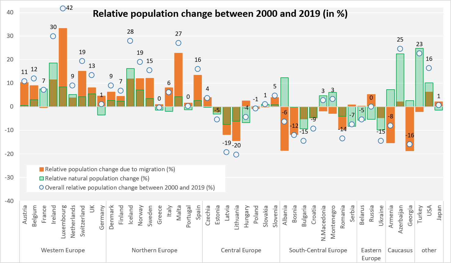
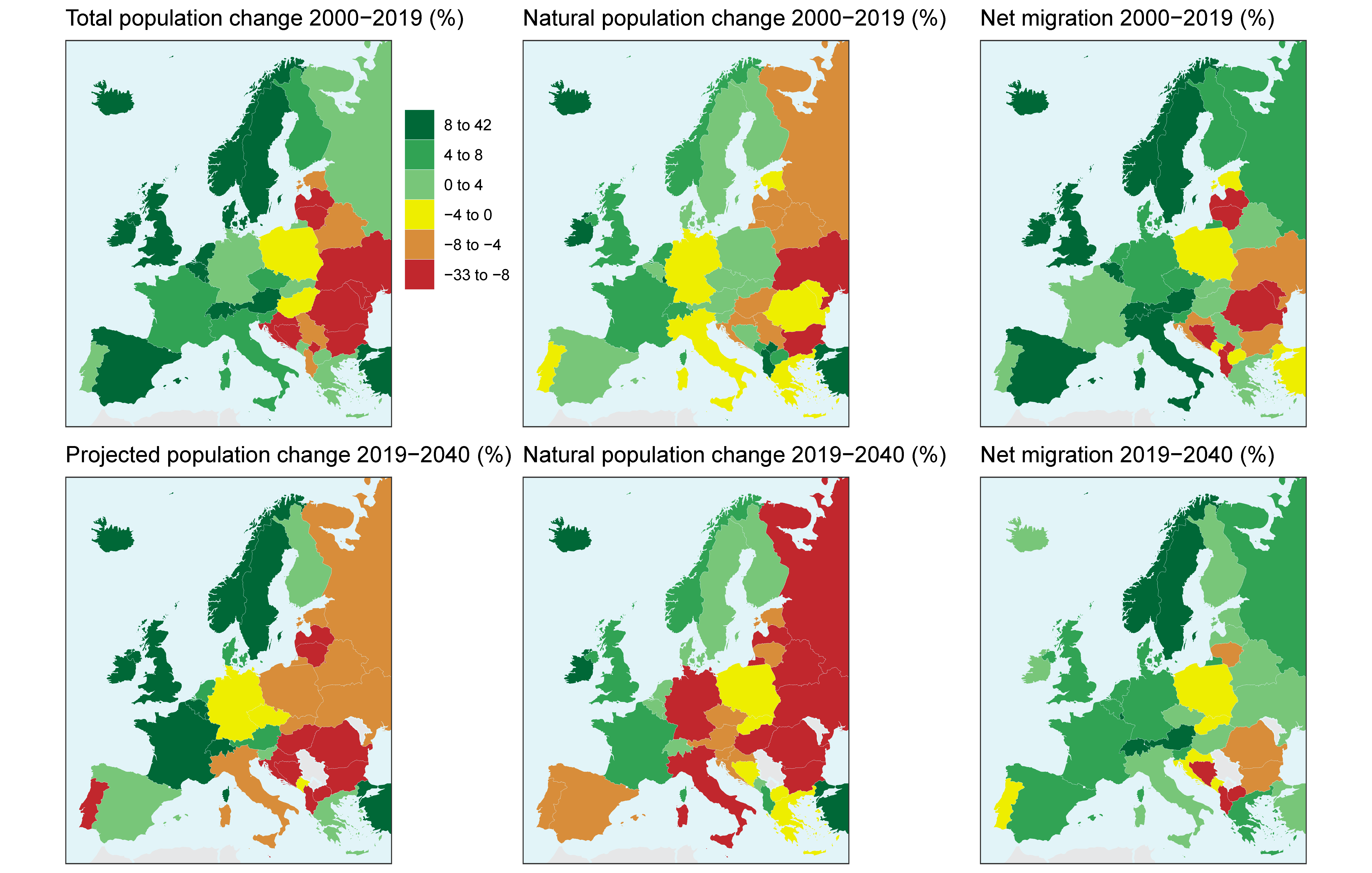
Europe remains divided by long-term population trends. This division mostly follows the past geopolitical cleavage between Europe’s East and West. Countries in the comparatively rich regions - the West, South, and North - continue to experience rising population, due to a combination of minor natural population increase and higher level of immigration than emigration. In contrast, almost all countries in Central, South-Eastern, and Eastern Europe saw substantial population declines, due to a combined effect of natural population decrease and emigration.

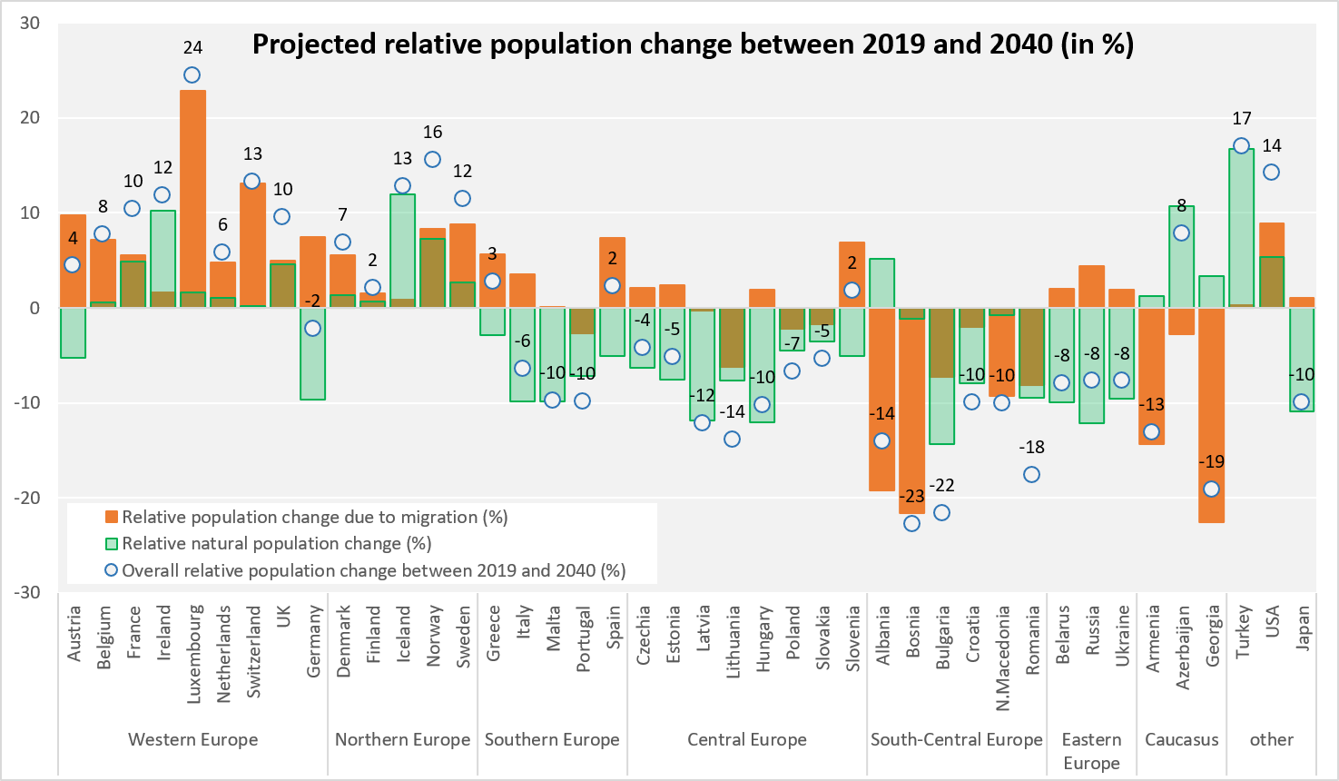
For the next 20 years, the population projections of the Wittgenstein Centre for Demography and Global Human Capital predict further continuation of these trends. Regional population balance will be affected by continuing migration from East to West, but also by increasing depopulation due to natural population change, not only in East but also in Central and Southern Europe and in Germany.

Figure Notes:
Figure 1: Relative population change between 2000 and 2019 (in %)
Figure 2: Projected relative population change between 2019 and 2040 (in %)
Figure 3: Observed and projected population trends in Europe, 2000–2040